Overview
My contributions to the #DuboisChallenge2024.
Data ready from the GitHub Repo
Download the georgia-1880-county-shapefile.zip file from: https://github.com/ajstarks/dubois-data-portraits/tree/master/challenge/2024/challenge01
georgia_shp <- sf::read_sf("data/georgia-1880-county-shapefile")

# georgia_shp%>%headdat_sf <- georgia_shp%>%
janitor::clean_names()%>%
separate(data1870,into=c("up70","down70"))%>%
separate(data1880_p,into=c("up80","down80"))%>%
mutate(# pop 1870
up70=ifelse(up70=="",0,up70),
down70=ifelse(is.na(down70),0,down70),
up70=as.numeric(up70),
down70=as.numeric(down70),
# pop 1880
up80=ifelse(up80=="",0,up80),
down80=ifelse(is.na(down80),0,down80),
up80=as.numeric(up80),
down80=as.numeric(down80))%>%
rowwise()%>%
mutate(pop70=mean(up70,down70),
pop80=mean(up80,down80))%>%
arrange(pop70,pop80)
data <- dat_sf%>%select(county=icpsrnam,
pop70,pop80)%>%
mutate(id=case_when(pop70 == 0 ~ 7,
pop70 == 1000 ~ 6,
pop70 == 2500 ~ 5,
pop70 == 5000 ~ 4,
pop70 == 10000 ~ 3,
pop70 == 15000 ~ 2,
pop70 == 20000 ~ 1),
pop70=case_when(pop70 == 0 ~ "UNDER 1,000",
pop70 == 1000 ~ "1000 TO 2,500",
pop70 == 2500 ~ "2,500 TO 5,000",
pop70 == 5000 ~ "5,000 TO 10,000",
pop70 == 10000 ~ "10,000 TO 15,000",
pop70 == 15000 ~ "15,000 TO 20,000",
pop70 == 20000 ~ "20,000 TO 30,000"))%>%
# pop80
mutate(id=case_when(pop80 == 0 ~ 7,
pop80 == 1000 ~ 6,
pop80 == 2500 ~ 5,
pop80 == 5000 ~ 4,
pop80 == 10000 ~ 3,
pop80 == 15000 ~ 2,
pop80 == 20000 ~ 1),
pop80=case_when(pop80 == 0 ~ "UNDER 1,000",
pop80 == 1000 ~ "1000 TO 2,500",
pop80 == 2500 ~ "2,500 TO 5,000",
pop80 == 5000 ~ "5,000 TO 10,000",
pop80 == 10000 ~ "10,000 TO 15,000",
pop80 == 15000 ~ "15,000 TO 20,000",
pop80 == 20000 ~ "20,000 TO 30,000"))
data%>%count(id,pop80)Dybois Style
Fonts:
library(sysfonts)
library(showtext)
sysfonts::font_add_google("Public Sans","Public Sans")
# font_add_google("Carter One", "Carter One")
showtext::showtext_auto()
showtext::showtext_opts(dpi=320)
Colors:
Background:
"#e7d6c5"Text:
c("#483c32","#bbaa98")legend_colors <- c("#372c59","#7a5039","#c29e84","#d63352",
"#e79d96","#edb456","#4b5c4f")Bounding box: xmin: 939223.1 ymin: -701249.8 xmax: 1425004 ymax: -200888.5
pop70_map <- data%>%
  ggplot()+
  geom_sf(aes(fill=pop70),
          show.legend = F,
          color="#483c32",alpha=0.9,
          linewidth=0.1)+
  scale_fill_manual(values=c("UNDER 1,000"="#4b5c4f",
                             "1000 TO 2,500"="#edb456",
                             "2,500 TO 5,000"="#e79d96",
                             "5,000 TO 10,000"="#d63352",
                             "10,000 TO 15,000"="#c29e84",
                             "15,000 TO 20,000"="#7a5039",
                             "20,000 TO 30,000"="#372c59"),na.value = "#e0cebb")+
    annotate("text", x = -84.45, y = 35.1,
           label = "1870",
           size = 3.5,color="#483c32",
           fontface = "bold",
           family =  "Public Sans" ) +
   coord_sf(crs=4326,clip = "off")+
  ggthemes::theme_map()+
  theme(plot.background = element_rect(color="#e7d6c5",fill="#e7d6c5"),
        panel.background = element_rect(color="#e7d6c5",fill="#e7d6c5"))

pop70_map
pop80_map <- data%>%
ggplot()+
geom_sf(aes(fill=pop80),
show.legend = F,
color="#483c32",alpha=0.9,
linewidth=0.1)+
scale_fill_manual(values=c("UNDER 1,000"="#4b5c4f",
"1000 TO 2,500"="#edb456",
"2,500 TO 5,000"="#e79d96",
"5,000 TO 10,000"="#d63352",
"10,000 TO 15,000"="#c29e84",
"15,000 TO 20,000"="#7a5039",
"20,000 TO 30,000"="#372c59"),na.value = "#e0cebb")+
annotate("text", x = -84.45, y = 35.1,
label = "1880",
size = 3.5,color="#483c32",
fontface = "bold",
family = "Public Sans" ) +
coord_sf(crs=4326,clip = "off")+
ggthemes::theme_map()+
theme(plot.background = element_rect(color="#e7d6c5",fill="#e7d6c5"),
panel.background = element_rect(color="#e7d6c5",fill="#e7d6c5"))
pop80_mapPlot layout
source: https://ggplot2-book.org/arranging-plots
pop70_map+ ggplot() + ggplot()+ pop80_map + plot_layout(ncol = 2,nrow = 2)legend1_plot <- legend1%>%
ggplot(aes(x,y))+
geom_point(aes(fill=label),
shape=21,stroke=0.1,
size=8.5,
show.legend = F)+
scale_fill_manual(values=c("5,000 TO 10,000"="#d63352",
"2,500 TO 5,000"="#e79d96",
"1000 TO 2,500"="#edb456",
"UNDER 1,000"="#4b5c4f"))+
geom_text(aes(label=label),
family="Public Sans",
size=3.5,color="#7a5039",
nudge_x = 0,hjust=-0.2)+
coord_cartesian(xlim=c(-0.2,1),ylim =c(-0,5) )+
ggthemes::theme_map()+
theme(plot.background = element_rect(color="#e7d6c5",fill="#e7d6c5"),
panel.background = element_rect(color="#e7d6c5",fill="#e7d6c5"))
legend1_plotlegend2_plot <- legend2%>%
ggplot(aes(x,y))+
geom_point(aes(fill=label),
shape=21,stroke=0.1,
size=8.5,
show.legend = F)+
scale_fill_manual(values=c("10,000 TO 15,000"="#c29e84",
"15,000 TO 20,000"="#7a5039",
"BETWEEN 20,000 AND 30,000"="#372c59"))+
geom_text(aes(label=label),
size=3.5,color="#7a5039",
family="Public Sans",
nudge_x = 0.5,hjust=0)+
coord_cartesian(xlim=c(-0.2,7),ylim =c(-1,4) )+
ggthemes::theme_map()+
theme(plot.background = element_rect(color="#e7d6c5",fill="#e7d6c5"),
panel.background = element_rect(color="#e7d6c5",fill="#e7d6c5"))
legend2_plotpop70_map+ legend2_plot + legend1_plot+ pop80_map + plot_layout(ncol = 2,nrow = 2)+plot_annotation(
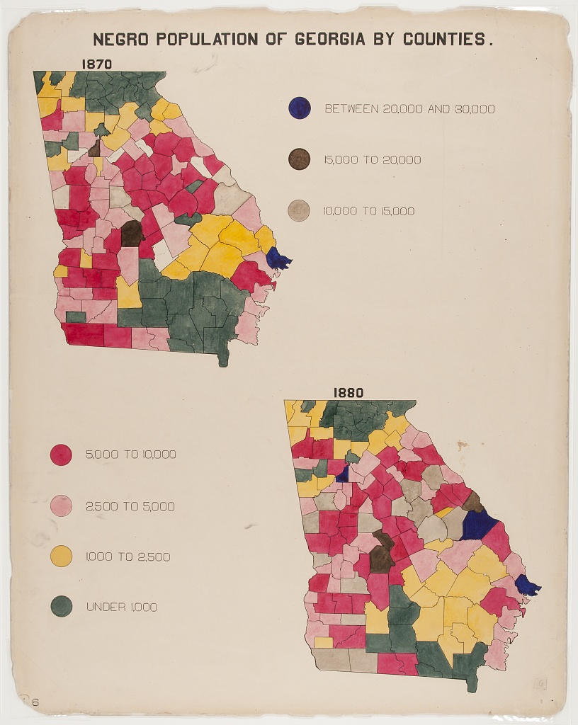
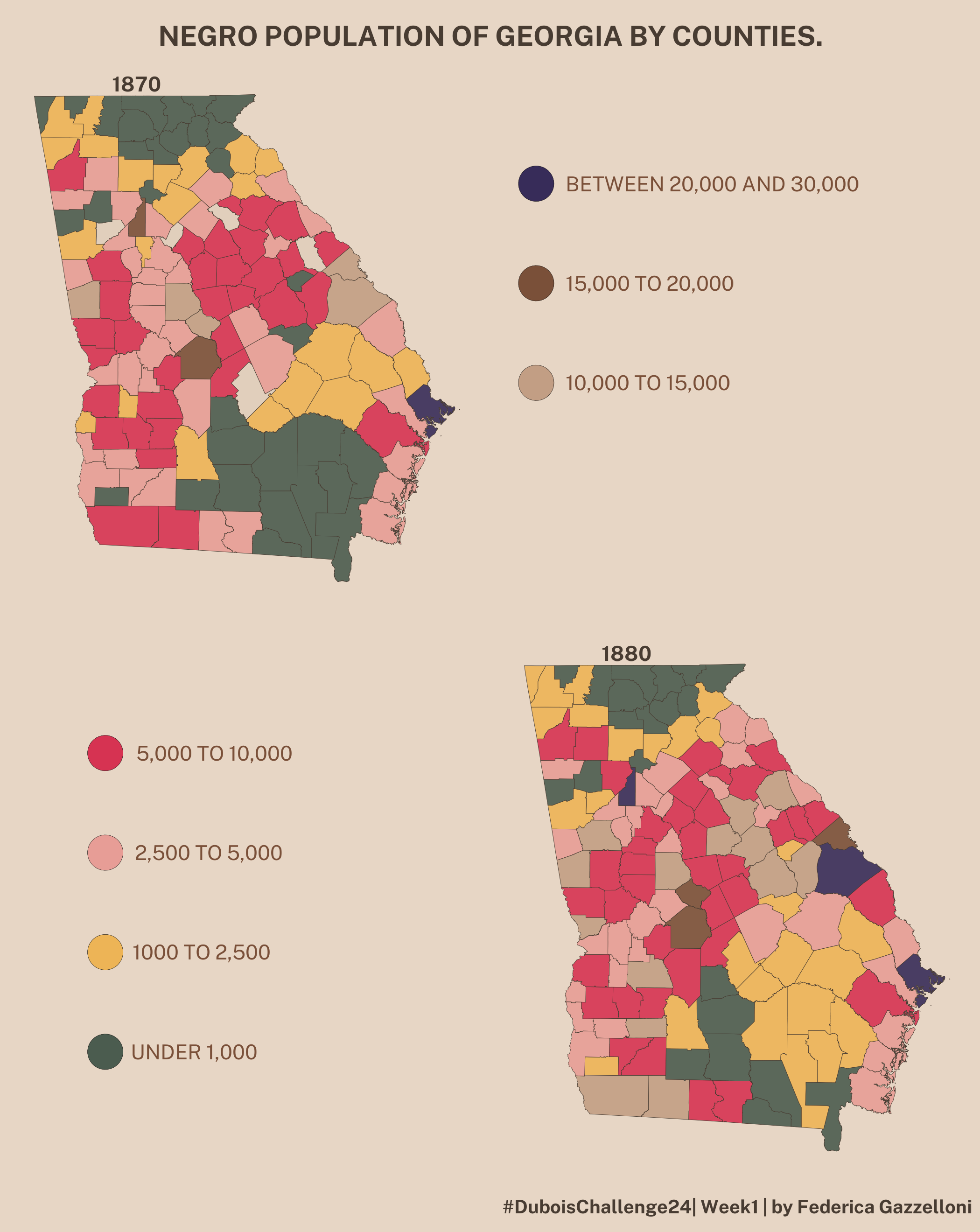
title = "NEGRO POPULATION OF GEORGIA BY COUNTIES.",
caption="#DuboisChallenge24| Week1 | by Federica Gazzelloni",
theme = theme_void(base_family = "Public Sans"))&
theme(text=element_text(color="#483c32",face="bold"),
plot.title = element_text(hjust=0.5),
plot.caption = element_text(size=9),
plot.background = element_rect(color="#e7d6c5",fill="#e7d6c5"),
panel.background = element_rect(color="#e7d6c5",fill="#e7d6c5"))ggsave("challenge01.png",bg="#e7d6c5",height = 8.8)