Asia

Overview

For this #30DayMapChallenge 2023 Day6 - Asia let’s explore the Population estimation for Regions and major Cities, from different sources.

Also, we will be looking at how to get started with {ggmap} to find the geocodes for the major cities in Asia.

Asia Cities and Population by Wikipedia.org

Let’s scrap the table of the Major Cities in Asia along with the Population level from Wikipedia.org.

Load the first set of libraries:

library(rvest)
library(stringr)
library(tidyverse)

html.population <- read_html('https://en.wikipedia.org/wiki/List_of_Asian_cities_by_population_within_city_limits')

df.asia_cities <- html.population %>%
  html_nodes("table") %>%
  .[[2]] %>%
  html_table(fill = TRUE)

df.asia_cities %>% names()

Select only the vectors of interest and clean data.

df.asia_cities <- df.asia_cities[-1,c(1,2,4)]

asia_cities <- df.asia_cities %>%
    mutate(Population = str_replace_all(Population, "\\[.*\\]","") %>% parse_number(),
           City_full= str_c(df.asia_cities$City, df.asia_cities$Nation, sep = ', ')) %>%
    select(City, Nation, City_full, Population)%>%
    filter(!str_detect(Nation,"Russia|Turkey"))


asia_cities %>% head()

Use GGMAP

To find the Asia City Geocodes we use the geocode() function from the {ggmap} package.

In order to get started with {ggmap} follow these steps:

• Install the package from source:

  remotes::install_github(“dkahle/ggmap”)

• Get started with Google Maps Platform https://developers.google.com/maps all you need to do, if you do not have access to the platform yet, is to get started a free trial by adding your bank account information (if you do not want to continue after the trials ends you can stop it without charges)

• Go to on the left-side bar menu and select Overview then ENABLE APIs

• Go to APIs & Services to check enabled APIs

• Go to Keys and Credentials and click +CREATE CREDENTIALS on the top-side bar

• Copy the API key and paste it in the register_google() function, the option write = T will save the credentials for future use in your .Renviron file:

  ggmap::register_google(, write = T)

Once you are all set try:

library(ggmap)

data.geo <- geocode(asia_cities$City_full)
data.geo%>%head

asia_cities_full <- cbind(asia_cities, data.geo)
# inspect
asia_cities_full %>% head() 

Mapping Asia Polygons

Let’s have a look at the map of Asia with {ggmap}.

map.asia <- get_map('Asia', zoom = 3)
map.asia %>% ggmap()

For this challenge we will be using another package for the polygons of Asia, the {rworldmap} package.

install.packages("rworldmap")

library(rworldmap)

worldmap <- rworldmap::getMap(resolution = "high")
dim(worldmap)

Have a look at the regions and choose Asia.

t(t(table(worldmap$REGION)))

asia <- worldmap[which(worldmap$REGION=="Asia"),]
asia%>%class

As it is a spatial polygon dataframe, and we’d like to use the geom_sf() function from the {ggplot2} package, we transform it to a simple feature object with st_as_sf() function from the {sf} package.

library(sf)

asia_sf <- asia %>%
  st_as_sf()

asia_sf %>% class()

Asia States by Population Level

To map the continent with population estimation by state we can set the option fill= POP_EST.

asia_sf %>%
  ggplot()+
  geom_sf(aes(fill=POP_EST))+
  scale_fill_continuous()

Population Level by custom class

Interesting is looking at a different classification of the population classes, and we do this by using the classIntervals() function from the {classInt} package for classifying the Population Estimation by quantile.

Let’s have a look at the population quantiles first. What we can see are the min and the max levels, and the values of the three quantiles, 25%, 50% (median), and the 75%. Which estimation of population follow in each quantile class.

The median population estimate for Asia is around 18 million, with some regions having populations of less than 1.5 billion people.

quantile(asia_sf$POP_EST, na.rm=TRUE)

asia_sf%>%
  ggplot(aes(POP_EST))+
  geom_histogram(aes(fill=SOVEREIGNT),bins = 20)+
  geom_vline(aes(xintercept = mean(POP_EST)),color="lightblue")+
  geom_vline(aes(xintercept = median(POP_EST)),color="midnightblue")+
  geom_text(aes(x=9000000,y=9,label="median"),size=2)+
  geom_text(aes(x=50000000,y=9,label="mean"),size=2)+
  scale_x_log10(labels=scales::comma_format(scale = 1/1000),n.breaks =8)+
  scale_fill_viridis_d()+
  labs(x="Population Estimation (Thousands)",
       title="Asia Population Distribution",
       caption="DataSource: {rworldmap} | Graphic: @fgazzelloni")+
  ggthemes::theme_clean()+
  theme(legend.text = element_text(size=5),
        legend.key.size = unit(5,units = "pt"))

We use the {classInt} package to find custom intervals of the population. And set up a new object called brks.

library(classInt)

brks <- classIntervals(asia_sf$POP_EST,
                       n=10, 
                       style="quantile")
brks

Set the color scheme:

brks <- brks$brks
colors <- RColorBrewer::brewer.pal(length(brks), "Spectral")

Finalize the dataset to use for the map with the population estimation interval cuts.

region_pop <- asia_sf%>%
  select(POP_EST)%>%
  mutate(breaks=case_when(POP_EST > 0 & POP_EST < 625493.5 ~ "[0,625493.5)",
                          POP_EST >= 625493.5 & POP_EST < 2691158 ~ "[625493.5,2691158)",
                          POP_EST >= 2691158 & POP_EST < 4728016 ~ "[2691158,4728016)",
                          POP_EST >= 4728016 & POP_EST < 6834942 ~ "[4728016,6834942)",
                          POP_EST >= 6834942 & POP_EST < 17788961 ~ "[6834942,17788961)",
                          POP_EST >= 17788961 & POP_EST < 23822783 ~ "[17788961,23822783)",
                          POP_EST >= 23822783 & POP_EST < 28625005 ~ "[23822783,28625005)",
                          POP_EST >= 28625005 & POP_EST < 65905410 ~ "[28625005,65905410)",
                          POP_EST >= 65905410 & POP_EST < 141564781 ~ "[65905410,141564781)",
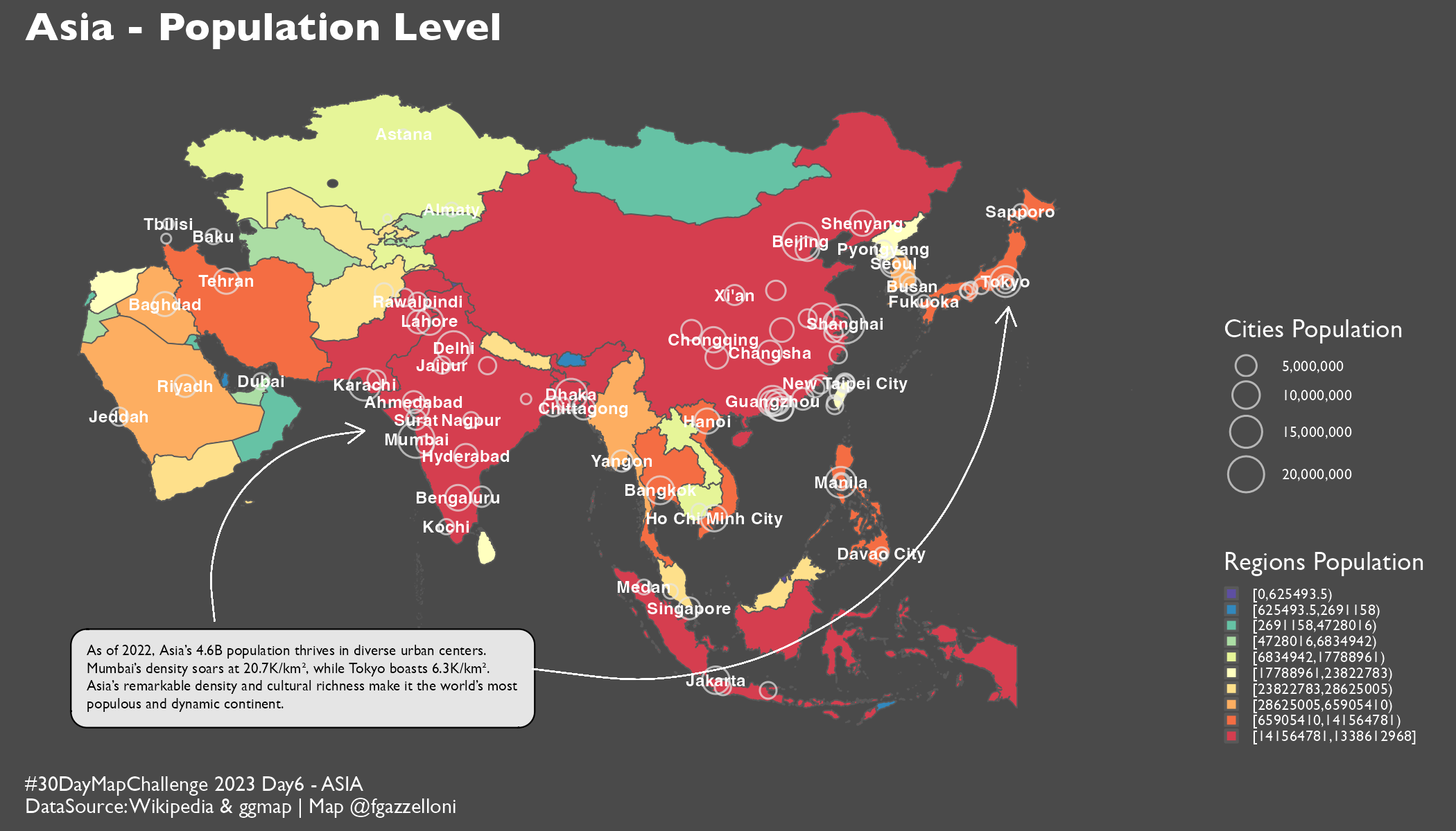
                          POP_EST >= 141564781 & POP_EST <= 1338612968 ~ "[141564781,1338612968]"))

Set some information about Asia Population on a text box with the geom_textbox() function from the {ggtext} package.

text <- tibble(asia_text=c("As of 2022, Asia's 4.6B population thrives in diverse urban centers. Mumbai's density soars at 20.7K/km², while Tokyo boasts 6.3K/km². Asia's remarkable density and cultural richness make it the world's most populous and dynamic continent."))

Make the Map

region_pop %>%
  ggplot()+
  geom_sf(aes(fill=breaks))+
  scale_fill_manual(breaks=c("[0,625493.5)","[625493.5,2691158)",
                               "[2691158,4728016)","[4728016,6834942)",
                             
                             "[6834942,17788961)","[17788961,23822783)",
                               "[23822783,28625005)","[28625005,65905410)",
                               "[65905410,141564781)","[141564781,1338612968]"),
                      values=rev(colors))+
  geom_point(data=asia_cities_full,
             mapping=aes(lon,lat,size=Population),
             shape=21,stroke=0.5,
             alpha=0.7,
             color="grey90",
             inherit.aes = F)+
  scale_size_continuous(labels=scales::comma_format())+
  geom_text(data=asia_cities_full,
             mapping=aes(lon,lat,label=City),fontface="bold",
            check_overlap = T,
            size=2.1,color="white")+
  ggtext::geom_textbox(data=text,
                       mapping=aes(x=60,y=-6,label=text),
                       size=1.8,width = 0.4,fill="grey90",
                       family = "Gill Sans",
                       inherit.aes = F)+
  geom_curve(x=50,xend=67,y=0,yend=20,
               linewidth=0.2,curvature = -0.5,
               arrow = arrow(angle=30, 
                             length = unit(0.1, "inches"),
                             ends = "last", type = "open"),
      color="white")+
    geom_curve(x=86,xend=140,y=-5,yend=33,
               linewidth=0.2,
               arrow = arrow(angle=30, 
                             length = unit(0.1, "inches"),
                             ends = "last", type = "open"),
      color="white")+
  labs(fill="Regions Population",
       size="Cities Population",
       title="Asia - Population Level",
       caption="#30DayMapChallenge 2023 Day6 - ASIA\nDataSource: Wikipedia & ggmap | Map @fgazzelloni")+
  ggthemes::theme_map()+
  theme(text=element_text(color="white", family = "Gill Sans"),
        plot.title = element_text(face="bold",size=14),
        plot.caption = element_text(hjust = 0),
        plot.background = element_rect(fill="#4A4A4A",color="#4A4A4A"),
        panel.background = element_rect(fill="#4A4A4A",color="#4A4A4A"),
        legend.background = element_blank(),
        legend.key = element_rect(color="#4A4A4A",fill="#4A4A4A"),
        legend.position = "right",
        legend.text = element_text(size=5.5),
        legend.key.size = unit(5.5,units = "pt"))

ggsave("day6_asia.png",
       width = 7,height = 4,
       bg="#4A4A4A")

Resources

• https://cran.r-project.org/web/packages/ggmap/readme/README.html
• https://www.r-bloggers.com/2017/09/mapping-the-largest-cities-in-asia-using-r/