library(tidyverse)
library(sf)
library(giscoR)
library(patchwork)
library(showtext)
font_add_google(name = 'Cormorant Garamond',
                family = 'Garamond')
showtext_auto()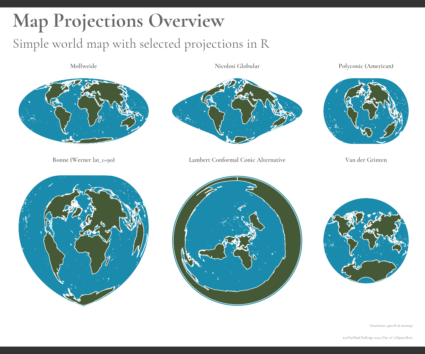
#sf::sf_proj_info()%>%View# Define common map projections
projections <- tibble::tibble(
proj_name = c("Mollweide", "Nicolosi Globular",
"Polyconic (American)", "Bonne (Werner lat_1=90)",
"Lambert Conformal Conic Alternative","Van der Grinten "),
crs = c(
"+proj=moll +datum=WGS84",
"+proj=nicol +datum=WGS84",
"+proj=poly +datum=WGS84",
"+proj=bonne lat_1=90",
"+proj=lcca lat_0=90",
"+proj=vandg lat_0=90"))projectionsSet the buffer for drawing the ocean.
# Define Earth radius and projection
earth_radius <- 6371000  # 6,371 km radius of Earth
# Step 1: Create an "ocean" layer (buffer around the Earth's center)
ocean <- st_point(c(0, 0)) %>%
  st_sfc(crs = 4326) %>%   # Define as a spatial feature
st_buffer(dist = earth_radius) ggplot() +
geom_sf(data = st_transform(ocean,
crs = "+proj=moll +datum=WGS84"),
fill = "#1a8bac", color = "white")# Create plots for each projection
projection_plots <- projections %>%
mutate(plot = purrr::map2(proj_name, crs, ~ {
ggplot() +
geom_sf(data = st_transform(ocean, crs = .y),
fill = "#1a8bac", color = "white") +
geom_sf(data = st_transform(gisco_coastallines, crs = .y),
fill = "#455936", color = "white") +
coord_sf() +
labs(title = .x) +
ggthemes::theme_map() +
theme(text = element_text(family = "Garamond",
color = "gray40"),,
plot.title = element_text(size = 16,
face = "bold",
hjust = 0.5),
plot.background = element_rect(fill = NA,
color = NA),
panel.background = element_rect(fill = NA,
color = NA),
axis.text = element_blank(),
axis.ticks = element_blank(),
panel.grid = element_blank()
)
}))projection_plotsoverview_plot <- wrap_plots(projection_plots$plot, ncol = 3) +
plot_annotation(title = "Overview of Common Map Projections",
subtitle = "Simple world map with various projections in R",
caption = "Source: Natural Earth | Created with ggplot2",
theme = theme(text = element_text(family = "Garamond",
color = "gray40"),
plot.title = element_text(size = 50,
face = "bold"),
plot.subtitle = element_text(size = 34,
color = "gray40")))
overview_plotCode for the final plot is locked. To unlock the code, please email: fede.gazzelloni@gmail.com