import pandas as pd
import sklearn as skFrom R to Python: A Gentle Introduction
Part 2: Python Libraries
Introduction
In this second part of the course, we will continue exploring Python syntax and libraries. We will cover more advanced topics, including data manipulation, visualization, and working with libraries like pandas and matplotlib. By the end of this part, you will have a solid understanding of how to use Python for data analysis and visualization.
Python Libraries
Python has a rich ecosystem of libraries that make it easy to perform data analysis and visualization. Some of the most popular libraries include:
pandas: A powerful library for data manipulation and analysis.matplotlib: A library for creating static, animated, and interactive visualizations in Python.seaborn: A library based onmatplotlibthat provides a high-level interface for drawing attractive statistical graphics.numpy: A library for numerical computing in Python, providing support for arrays and matrices.scikit-learn: A library for machine learning in Python, providing simple and efficient tools for data mining and data analysis.statsmodels: A library for estimating and testing statistical models in Python.- and many more!
Installing Libraries
To install a library in Python, you can use the pip package manager. Open a terminal and type the following command:
pip install library_nameFor example, to install the pandas or scikit-learn library, you can use the following command:
pip install pandas
pip install scikit-learn
Then restart your Python session to use the newly installed library.
You can also install multiple libraries at once by separating them with spaces:
pip install pandas scikit-learn matplotlib seabornLoading Libraries
To use a library in Python, you need to import it first. You can do this using the import statement. You can also give a library an alias using the as keyword. This is useful for shortening long library names. For example, to import the pandas library. and give it the alias pd, you can use the following code:
The scikit-learn library is often imported as sklearn, and use the alias sk for convenience.
You can also import specific functions or classes from a library using from and import keywords. For example, to import the datasets class from the sklearn library, you can use the following code:
from sklearn import datasets

# Load the famous 'iris' dataset
iris = datasets.load_iris()
A tab completion feature is available in most IDEs, which can help you find the correct function names and their parameters. This is similar to the ? operator in R, which provides help on functions and datasets.
Another way to use a function from a package that is loaded is to the alias of the package followed by a dot and the function name. For example, to use the DataFrame function from the pandas package, you can use the following code:
# Convert it into a pandas DataFrame for easy manipulation
df_iris = pd.DataFrame(iris.data, columns=iris.feature_names)
The .head() method is used to display the first few rows of the DataFrame. This is similar to the head() function in R, which displays the first few rows of a data frame.
df_iris.head()| sepal length (cm) | sepal width (cm) | petal length (cm) | petal width (cm) | |
|---|---|---|---|---|
| 0 | 5.1 | 3.5 | 1.4 | 0.2 |
| 1 | 4.9 | 3.0 | 1.4 | 0.2 |
| 2 | 4.7 | 3.2 | 1.3 | 0.2 |
| 3 | 4.6 | 3.1 | 1.5 | 0.2 |
| 4 | 5.0 | 3.6 | 1.4 | 0.2 |
Reading Data
To read csv data, for example, you can use the read_csv() function from the pandas library. For example, to read a CSV file named data.csv, you can use the following code:
df = pd.read_csv("data.csv")This will store it in a DataFrame object called df. You can then use various functions and methods provided by the pandas library to manipulate and analyze the data in the DataFrame.
Data Manipulation with pandas
pandas is a powerful library for data manipulation and analysis. It provides data structures like Series and DataFrame, which are similar to R’s vectors and data frames, respectively. In this section, we will cover some basic data manipulation techniques using pandas.
Ready-to-Use Datasets
| Python | R | |
|---|---|---|
| Main packages | seaborn, sklearn.datasets, statsmodels.datasets |
datasets (built-in), MASS, ISLR, palmerpenguins, ggplot2movies |
| How to load | sns.load_dataset('iris'), sklearn.datasets.load_diabetes() |
data(iris), data(mtcars), data(airquality) |
| Examples of datasets | Iris, Titanic, Boston Housing, MNIST | Iris, Titanic, mtcars, airquality, CO2 |
| Additional datasets | Huggingface datasets package for ML, UCI datasets (scikit-learn) |
dslabs::gapminder, nycflights13, palmerpenguins |
Creating a Custom DataFrame
You can create a DataFrame in pandas using the DataFrame() constructor. For example, to create a DataFrame from a dictionary, you can use the following code:
data = {
    "Name": ["Alice", "Bob", "Charlie"],
    "Age": [25, 30, 35],
    "City": ["New York", "Los Angeles", "Chicago"]
}
df = pd.DataFrame(data)
df| Name | Age | City | |
|---|---|---|---|
| 0 | Alice | 25 | New York |
| 1 | Bob | 30 | Los Angeles |
| 2 | Charlie | 35 | Chicago |
Accessing Data
You can access data in a DataFrame using the column names or indices. For example, to access the “Name” column, you can use the following code:
df["Name"]0 Alice
1 Bob
2 Charlie
Name: Name, dtype: objectYou can also access multiple columns by passing a list of column names:
df[["Name", "City"]]| Name | City | |
|---|---|---|
| 0 | Alice | New York |
| 1 | Bob | Los Angeles |
| 2 | Charlie | Chicago |
You can access rows using the iloc method, which allows you to specify the row indices.
Ask for help:
help(df.iloc)For example, to access the first row, you can use the following code:
df.iloc[0]Name Alice
Age 25
City New York
Name: 0, dtype: objectIn Python , indexing starts at 0, so the first row is at index 0, the second row is at index 1, and so on.
Filtering Data
You can filter data in a DataFrame using boolean indexing. For example, to filter rows where the “Age” column is greater than 30, you can use the following code:
filtered_df = df[df["Age"] > 30]
filtered_df| Name | Age | City | |
|---|---|---|---|
| 2 | Charlie | 35 | Chicago |
You can also use multiple conditions to filter data. For example, to filter rows where the “Age” column is greater than 30 and the “City” column is “Los Angeles”, you can use the following code:
filtered_df = df[(df["Age"] > 30) & (df["City"] == "Los Angeles")]
filtered_df| Name | Age | City |
|---|
Adding and Removing Columns
You can add a new column to a DataFrame by assigning a value to a new column name. For example, to add a new column called “Salary”, you can use the following code:
df["Salary"] = [50000, 60000, 70000]
df| Name | Age | City | Salary | |
|---|---|---|---|---|
| 0 | Alice | 25 | New York | 50000 |
| 1 | Bob | 30 | Los Angeles | 60000 |
| 2 | Charlie | 35 | Chicago | 70000 |
You can also remove a column using the drop() method. For example, to remove the “Salary” column, you can use the following code:
df = df.drop("Salary", axis=1)
df| Name | Age | City | |
|---|---|---|---|
| 0 | Alice | 25 | New York |
| 1 | Bob | 30 | Los Angeles |
| 2 | Charlie | 35 | Chicago |
Renaming Columns
You can rename columns in a DataFrame using the rename() method. For example, to rename the “Name” column to “First Name”, you can use the following code:
df = df.rename(columns={"Name": "First Name"})
df| First Name | Age | City | |
|---|---|---|---|
| 0 | Alice | 25 | New York |
| 1 | Bob | 30 | Los Angeles |
| 2 | Charlie | 35 | Chicago |
Sorting Data
You can sort a DataFrame using the sort_values() method. For example, to sort the DataFrame by the “Age” column in ascending order, you can use the following code:
df = df.sort_values(by="Age")
df| First Name | Age | City | |
|---|---|---|---|
| 0 | Alice | 25 | New York |
| 1 | Bob | 30 | Los Angeles |
| 2 | Charlie | 35 | Chicago |
You can also sort by multiple columns by passing a list of column names:
df = df.sort_values(by=["City", "Age"])
df| First Name | Age | City | |
|---|---|---|---|
| 2 | Charlie | 35 | Chicago |
| 1 | Bob | 30 | Los Angeles |
| 0 | Alice | 25 | New York |
Grouping Data
You can group data in a DataFrame using the groupby() method. For example, to group the DataFrame by the “City” column and calculate the mean age for each city, you can use the following code:
df_animals = pd.DataFrame({'Animal': ['Falcon', 'Falcon', 'Parrot', 'Parrot'],'Max Speed': [380., 370., 24., 26.]})

df_animals| Animal | Max Speed | |
|---|---|---|
| 0 | Falcon | 380.0 |
| 1 | Falcon | 370.0 |
| 2 | Parrot | 24.0 |
| 3 | Parrot | 26.0 |
Gain some help with:
help(df.groupby)df_animals.groupby(['Animal']).mean()| Max Speed | |
|---|---|
| Animal | |
| Falcon | 375.0 |
| Parrot | 25.0 |
Aggregating Data
You can aggregate data in a DataFrame using the agg() method. For example, to calculate the mean and sum of the “Age” column for each city, you can use the following code:
aggregated_df = df.groupby("City").agg({"Age": ["mean", "sum"]})
aggregated_df| Age | ||
|---|---|---|
| mean | sum | |
| City | ||
| Chicago | 35.0 | 35 |
| Los Angeles | 30.0 | 30 |
| New York | 25.0 | 25 |
Merging DataFrames
You can merge two DataFrames using the merge() method. For example, to merge two DataFrames on a common column, you can use the following code:
df1 = pd.DataFrame({"ID": [1, 2, 3], "Name": ["Alice", "Bob", "Charlie"]})
df2 = pd.DataFrame({"ID": [1, 2, 3], "Age": [25, 30, 35]})
merged_df = pd.merge(df1, df2, on="ID")
merged_df| ID | Name | Age | |
|---|---|---|---|
| 0 | 1 | Alice | 25 |
| 1 | 2 | Bob | 30 |
| 2 | 3 | Charlie | 35 |
Concatenating DataFrames
You can concatenate two or more DataFrames using the concat() function. For example, to concatenate two DataFrames vertically, you can use the following code:
df1 = pd.DataFrame({"Name": ["Alice", "Bob"], "Age": [25, 30]})
df2 = pd.DataFrame({"Name": ["Charlie", "David"], "Age": [35, 40]})
concatenated_df = pd.concat([df1, df2], ignore_index=True)
concatenated_df| Name | Age | |
|---|---|---|
| 0 | Alice | 25 |
| 1 | Bob | 30 |
| 2 | Charlie | 35 |
| 3 | David | 40 |
Pivoting Data
You can pivot a DataFrame using the pivot() method. For example, to pivot a DataFrame based on two columns, you can use the following code:
df = pd.DataFrame({
    "Date": ["2023-01-01", "2023-01-01", "2023-01-02", "2023-01-02"],
    "Category": ["A", "B", "A", "B"],
    "Value": [10, 20, 30, 40]
})
pivoted_df = df.pivot(index="Date", columns="Category", values="Value")
pivoted_df| Category | A | B |
|---|---|---|
| Date | ||
| 2023-01-01 | 10 | 20 |
| 2023-01-02 | 30 | 40 |
Reshaping Data
You can reshape a DataFrame using the melt() method. For example, to reshape a DataFrame from wide format to long format, you can use the following code:
df = pd.DataFrame({
    "ID": [1, 2, 3],
    "Name": ["Alice", "Bob", "Charlie"],
    "Age": [25, 30, 35]
})
reshaped_df = pd.melt(df, id_vars=["ID"], value_vars=["Name", "Age"])
reshaped_df| ID | variable | value | |
|---|---|---|---|
| 0 | 1 | Name | Alice |
| 1 | 2 | Name | Bob |
| 2 | 3 | Name | Charlie |
| 3 | 1 | Age | 25 |
| 4 | 2 | Age | 30 |
| 5 | 3 | Age | 35 |
Handling Missing Data
You can handle missing data in a DataFrame using the isnull() and dropna() methods. For example, to check for missing values in a DataFrame, you can use the following code:
df = pd.DataFrame({"Name": ["Alice", None, "Charlie"], "Age": [25, 30, None]})
df.isnull()| Name | Age | |
|---|---|---|
| 0 | False | False |
| 1 | True | False |
| 2 | False | True |
You can also drop rows with missing values using the dropna() method:
df = df.dropna()
df| Name | Age | |
|---|---|---|
| 0 | Alice | 25.0 |
Saving Data
You can save a DataFrame to a CSV file using the to_csv() method. For example, to save the DataFrame to a file named output.csv, you can use the following code:
df.to_csv("output.csv", index=False)You can also save a DataFrame to other formats, such as Excel, JSON, and SQL databases, using the appropriate methods provided by pandas.
Data Visualization
matplotlib is a powerful library for creating static, animated, and interactive visualizations in Python. It provides a wide range of plotting functions and customization options. In this section, we will cover some basic plotting techniques using matplotlib.
You can create a simple line plot using the plot() function. For example, to create a line plot of the x and y values, you can use the following code:
import matplotlib.pyplot as plt
import numpy as np
x = np.linspace(0, 10, 100)
y = np.sin(x)
plt.plot(x, y)
plt.xlabel("X-axis")
plt.ylabel("Y-axis")
plt.title("Sine Wave")
plt.show()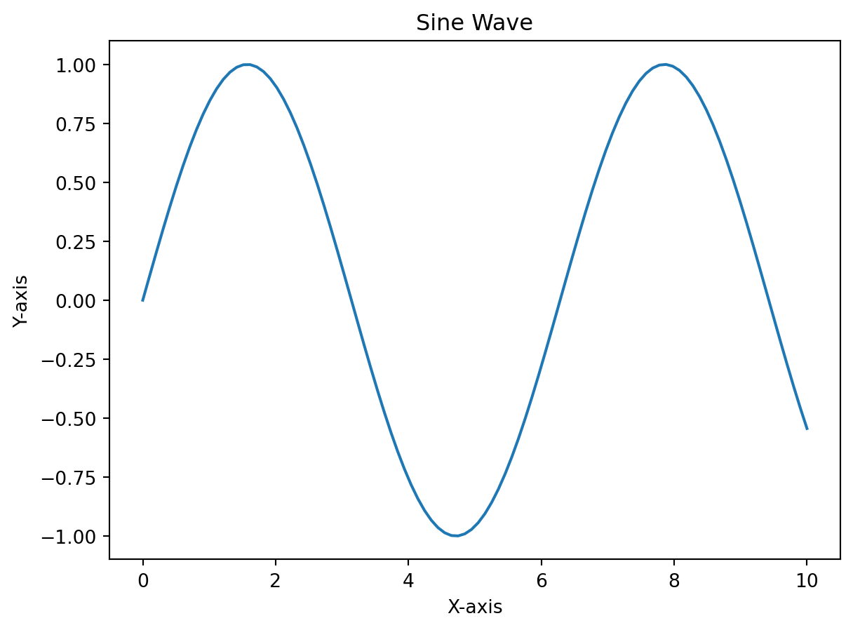
As in R we have ggplot2, in Python we have seaborn, which is a high-level interface for drawing attractive statistical graphics. It is built on top of matplotlib and provides a more user-friendly API for creating complex visualizations.
Install seaborn using pip:
pip install seabornThen load the library in your Python script:
import seaborn as snssns.set(style="whitegrid")
tips = sns.load_dataset("tips")
sns.scatterplot(x="total_bill", y="tip", data=tips)
plt.show()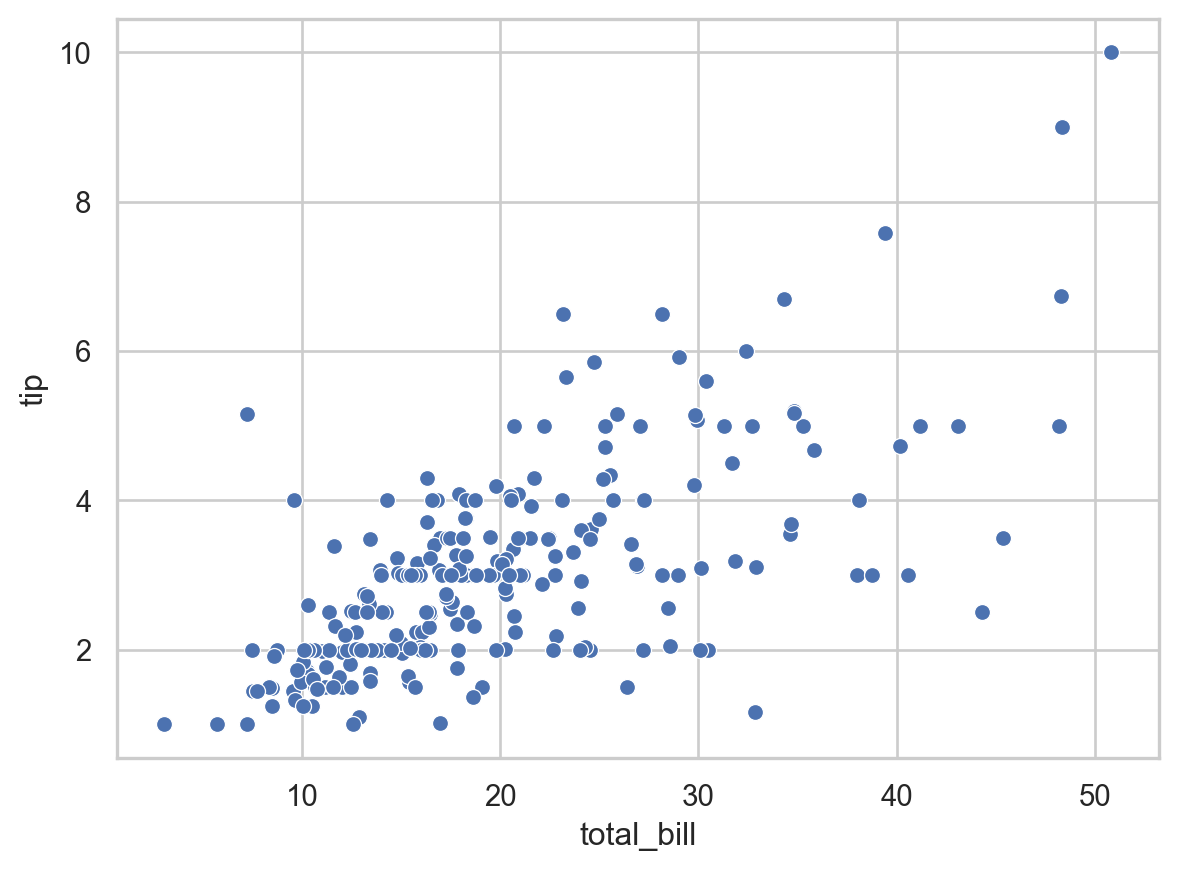
Conclusion
In course, we have covered the basics of Python syntax and libraries. We have also explored some advanced topics, such as merging and reshaping data. By now, you should have a solid understanding of how to use Python for data analysis and visualization.
This booklet is made in quarto, a scientific and technical publishing system built on Pandoc, where you can use both R and Python code chunks in the same document. It is similar to R Markdown, but with more features and flexibility. You can find more information about quarto at https://quarto.org.