Appendix C — Tips on Converting to Python

Translating R code into Python can be a smooth transition with the right approach. Let’s start with the basics, from installing packages to loading libraries, and compare the equivalents between R and Python, including the popular tidyverse in R and its counterparts in Python.

C.1 Packages and Libraries

Installing Packages:

R:
```
install.packages("package_name")
```
Python (using pip):
```
!pip install package_name
```
Python (using conda):
```
!conda install package_name
```

Loading Libraries:

R:
```
library(package_name)
```
Python:
```
import package_name
```

C.2 Comparing tidyverse with its Python Equivalents

tidyverse (R): tidyverse is a collection of R packages designed for data science, including dplyr for data manipulation, ggplot2 for data visualization, tidyr for data tidying, etc.
```
library(tidyverse)
```
Python Equivalents:
- pandas: Similar to dplyr, pandas provides powerful data manipulation tools.
```
import pandas as pd
```
- matplotlib/seaborn: Comparable to ggplot2, these libraries are used for data visualization.
```
import matplotlib.pyplot as plt
import seaborn as sns
```
- numpy: While not a direct equivalent to tidyr, numpy offers functionalities for array manipulation and numerical computing, which can be handy for data tidying tasks.
```
import numpy as np
```
- scikit-learn: Provides tools for data preprocessing, modelling, and evaluation, resembling some functionalities of tidyverse packages like modelr.
```
from sklearn import ...
```
- tidyverse-like package: There isn’t a single package in Python that encompasses the entire functionality of tidyverse, but you can combine pandas, matplotlib/seaborn, numpy, and scikit-learn to achieve similar results.

By understanding these equivalences and leveraging the rich ecosystem of Python libraries, you can effectively translate your R code into Python, ensuring a smooth transition while retaining the analytical power and flexibility you need for your projects.

C.3 Creating Data Making Statistics

Creating Basic Data:

# Create a data frame
data <- data.frame(
  x = c(1, 2, 3, 4, 5),
  y = c(2, 3, 4, 5, 6)
)

Python (using pandas):

import pandas as pd

# Create a DataFrame
data = pd.DataFrame({
    'x': [1, 2, 3, 4, 5],
    'y': [2, 3, 4, 5, 6]
})

Basic Statistics:

R:
```
# Summary statistics
summary(data)
```

Python (using pandas):

# Summary statistics
print(data.describe())

C.4 Building a Linear Regression Model

# Load the lm function from the stats package
library(stats)

# Fit a linear regression model
lm_model <- lm(y ~ x, data = data)

# Summary of the model
summary(lm_model)

Python (using statsmodels):

import statsmodels.api as sm

# Add a constant term for intercept
X = sm.add_constant(data['x'])

# Fit a linear regression model
lm_model = sm.OLS(data['y'], X).fit()

# Summary of the model
print(lm_model.summary())

Python (using scikit-learn):

from sklearn.linear_model import LinearRegression

# Initialize the model
lm_model = LinearRegression()

# Fit the model
lm_model.fit(data[['x']], data['y'])

# Coefficients
print("Intercept:", lm_model.intercept_)
print("Coefficient:", lm_model.coef_)

While the syntax and libraries may differ slightly, the overall process remains conceptually similar. By understanding these comparisons, you can effectively transition between R and Python for data analysis and modelling tasks.

C.5 Example of a Model Workflow

Data Preprocessing:

import pandas as pd
from sklearn.preprocessing import StandardScaler
data = pd.read_csv('data.csv')
data.fillna(method='ffill', inplace=True)  
scaler = StandardScaler()
scaled_data = scaler.fit_transform(
  data[['feature1', 'feature2', 'feature3']]
  )

Model Selection and Training:

from sklearn.model_selection import train_test_split
from sklearn.linear_model import LinearRegression
from sklearn.metrics import mean_squared_error

X = data[['feature1', 'feature2', 'feature3']]
y = data['DALYs']
X_train, 
X_test, 
y_train, 
y_test = train_test_split(X, y, test_size=0.2, random_state=42)

model = LinearRegression()
model.fit(X_train, y_train)
y_pred = model.predict(X_test)

mse = mean_squared_error(y_test, y_pred)
print(f'Mean Squared Error: {mse}')

Time Series Forecasting Example:

from fbprophet import Prophet
ts_data = data[['date', 'DALYs']]
ts_data.rename(columns={'date': 'ds', 'DALYs': 'y'}, inplace=True)
model = Prophet()
model.fit(ts_data)
future = model.make_future_dataframe(periods=365)
forecast = model.predict(future)
model.plot(forecast)

The SIR Model Example:

Set-up the environment for running python in RStudio by loading the {reticulate} package and the following commands:

library(reticulate)

This is to configurate python and for installing necessary packages:

py_config()

# type <pip3 install scipy> on terminal
# type <pip3 install matplotlib> on terminal

import matplotlib
matplotlib.use('TkAgg')  # Ensure you have an interactive backend
import matplotlib.pyplot as plt
import scipy.integrate as spi
import numpy as np

Set-up the parameters:

beta = 1.4247
gamma = 0.14286
TS = 1.0
ND = 70.0
S0 = 1 - 1e-6
I0 = 1e-6
INPUT = (S0, I0, 0.0)

Define differential equations:

def diff_eqs(INP, t):
    Y = np.zeros((3))
    V = INP
    Y[0] = - beta * V[0] * V[1]
    Y[1] = beta * V[0] * V[1] - gamma * V[1]
    Y[2] = gamma * V[1]
    return Y

t_start = 0.0; t_end = ND; t_inc = TS
t_range = np.arange(t_start, t_end + t_inc, t_inc)
RES = spi.odeint(diff_eqs, INPUT, t_range)

#Plotting
# Ensure interactive mode is on and plot
plt.ion()
plt.subplot(211)
plt.plot(RES[:, 0], '-g', label='Susceptibles')
plt.plot(RES[:, 2], '-k', label='Recovereds')
plt.legend(loc=0)
plt.title('SIR Model')
plt.xlabel('Time')
plt.ylabel('Susceptibles and Recovereds')

plt.subplot(212)
plt.plot(RES[:, 1], '-r', label='Infectious')
plt.xlabel('Time')
plt.ylabel('Infectious')

plt.show()

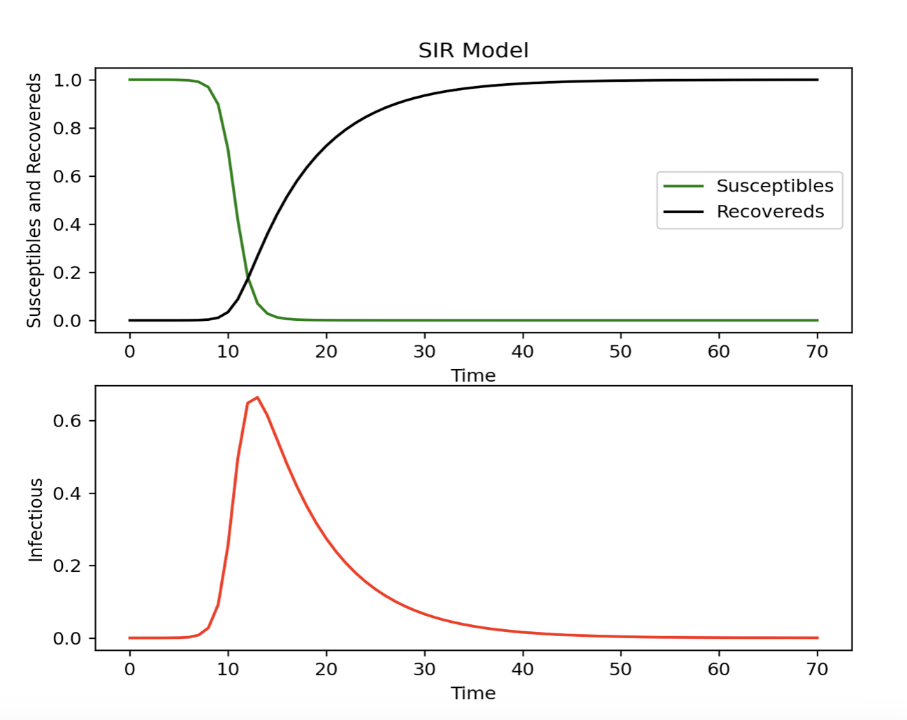
The code for this example is adapted from: Modeling Infectious Diseases in Humans and Animals Matt J. Keeling & Pejman Rohani.

By following these steps, you can analyze DALYs and infectious diseases, drawing trends, understanding relationships, and predicting future outcomes effectively.